import distl
import numpy as np
Unless cache_sample=False is passed, calling sample will cache the results so that successive calls to pdf, logpdf, cdf, logcdf, etc are computed based on the latest sampled values. This avoids the need to do the following:
samples = dist.sample()
print(samples)
dist.pdf(samples)
Although this wouldn't exactly be difficult for a simple univariate and even multivariate cases... things get a lot more complicated with MultivariateSlice, Composite, and DistributionCollections. distl allows for tracking the samples of the underlying distributions, but it is important to understand when covariances are respected and when they're ignored.
Univariate Distributions
g = distl.gaussian(10, 2, label='g')
g.sample()
9.721287674158706
g.cached_sample
9.721287674158706
g.pdf()
0.19754363470337227
If passing size to sample then the cached values will keep that shape and pdf etc will return an array with one entry per sample.
g.sample(size=2)
array([9.98849481, 8.82841238])
g.cached_sample
array([9.98849481, 8.82841238])
g.pdf()
array([0.19946784, 0.16802157])
Of course at any point a value can be passed to any of this methods to override computing at the cached sample values.
g.pdf(10.5)
0.19333405840142465
Multivariate Distributions
Multivariate distributions essentially act the same as Univariate distributions except the returned samples have an extra dimension. The provided covariances are always respected - calls to pdf etc return the probability of drawing the provided set of values from the multivariate distribution.
mvg = distl.mvgaussian([5,10, 12],
                       np.array([[ 2,  1, -1],
                                 [ 1,  2,  1],
                                 [-1,  1,  2]]),
                       allow_singular=True,
                       labels=['a', 'b', 'c'])
mvg.sample()
array([ 6.00852787, 10.80919367, 11.80066581])
mvg.cached_sample.shape[-1], mvg.ndimensions
(3, 3)
For multivariates, pdf is the probability density of drawing the set of values for each dimension.
mvg.pdf()
0.03988457910748257
If passing size to sample, then the samples will be of shape (size, ndimensions) and the pdf call will return an array with length size.
mvg.sample(size=2)
array([[ 3.58096794,  8.73594357, 12.15497563],
       [ 3.39273776,  8.2082576 , 11.81551984]])
mvg.cached_sample
array([[ 3.58096794,  8.73594357, 12.15497563],
       [ 3.39273776,  8.2082576 , 11.81551984]])
mvg.pdf()
array([0.02894357, 0.0200853 ])
MultivariateSlice Distributions
It is important to remember that MultivariateSlices act as Univariate distributions for all cases except sampling - in which case the covariances can be remembered. This allows for a lot of convenience functionality such as plotting the projected pdf. That said - since the underlying distribution is a multivariate, the multivariate probabilities can still be manually accessed.
mvg_a = mvg.slice('a')
mvg_a.sample()
2.545541526091035
mvg_a.cached_sample
2.545541526091035
mvg_a.multivariate.cached_sample
array([ 2.54554153, 7.27949851, 11.73395698])
A call to pdf will expose the pdf of the flattened univariate representation of this slice given cached_sample above.
mvg_a.pdf()
0.06256159274936313
Note the important distinction between the line above and the one below. Below we are accessing the probability of drawing the set of drawn values (from mvg_a.multivariate.cached_sample).
mvg_a.multivariate.pdf()
0.0055950763249043205
As in the other cases, this same logic applies when passing size to sample.
mvg_a.sample(size=2)
array([5.42603723, 5.64367394])
mvg_a.cached_sample
array([ 5.42603723, 10.2365534 , 11.81051617])
mvg_a.pdf()
array([2.69580279e-01, 2.97265466e-04, 2.59663353e-06])
Composite Distributions
Similarly to MultivariateSlices, Composite distributions also expose the univariate pdfs after any math operations, but use the underlying "children" distributions when sampling to respect any covariances.
g = distl.gaussian(10, 2, label='g')
u = distl.uniform(1, 3, label='u')
c = g * u
c.sample()
33.66343441962413
c.cached_sample
33.66343441962413
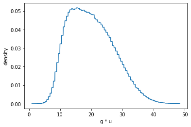
As with MultivariateSlices, pdf here is exposing the probability of drawing cached_sample (or the provided value) from the combined/flattened distribution.
c.pdf()
0.010498210198406919
where the pdf is being determined from the stored (interpolated) flattened pdf function.
out = c.plot_pdf(show=True)
However, the underlying drawn values of the children distributions are still accessible. Here we can see the values for the gaussian and uniform distributions that were drawn before applying multiplication.
c.cached_sample_children
array([11.33333681, 2.97030213])
c.cached_sample_children[0] * c.cached_sample_children[1]
33.66343441962413
If we wanted to, we could determine the individual probabilities of drawing these two components.
c.dists[0].pdf(c.cached_sample_children[0]), c.dists[1].pdf(c.cached_sample_children[1])
(0.15972381785375794, 0.5)
The probability of drawing this set of values from the children would then be the product (or the sum in the case of logpdf).
c.dists[0].pdf(c.cached_sample_children[0]) * c.dists[1].pdf(c.cached_sample_children[1])
0.07986190892687897
As you probably expect by now, the same logic holds when passing size to sample.
c.sample(size=2)
array([33.66343442, 13.27444812])
c.cached_sample
array([33.66343442, 13.27444812])
c.cached_sample_children
array([[11.33333681, 11.55150092],
       [ 2.97030213,  1.14915354]])
Distribution Collection
dc = distl.DistributionCollection(g, mvg_a, c)
dc
<distl.distl.DistributionCollection at 0x7f6cdf400f10>
dc.sample()
array([10.29324649, 1.80357226, 13.51681186])
For collections, cached_sample refers to the passed distributions...
dc.cached_sample
array([10.29324649, 1.80357226, 13.51681186])
dc.labels
['g', 'a', 'g * u']
... whereas cached_samples_unpacked refers to the unpacked list of all underlying distributions (i.e. composite distributions are broken down into their subcomponents so that all the actual drawn values can be recorded to track covariances).
dc.cached_sample_unpacked
array([10.29324649, 1.80357226, 10.29324649, 1.31317285])
dc.labels_unpacked
['g', 'a', 'g', 'u']
We can notice a few things here. The first is that u shows up twice (as it is returned in the sample but also used in the math to compute c), and is given the same value in both cases. Furthermore, c was defined as g * u, which we can confirm here by doing math on the cached values.
dc.cached_sample_unpacked[2] * dc.cached_sample_unpacked[3], dc.cached_sample[2]
(13.516811861939296, 13.516811861939296)
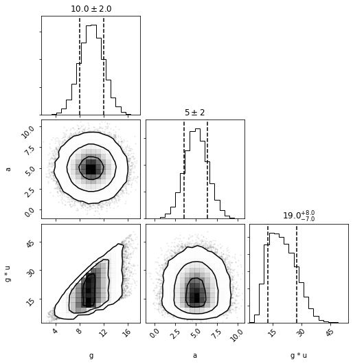
We can also see that the covariances are respected by plotting. For more details, see the DistributionCollections examples.
out = dc.plot(show=True)
Now if we rely on the cached values when calling pdf it will default to passing cached_sample_unpacked (and ignoring duplicate entries when doing the sum/product), therefore accounting for covariances.
dc.cached_sample
array([10.29324649, 1.80357226, 13.51681186])
dc.cached_sample_unpacked
array([10.29324649, 1.80357226, 10.29324649, 1.31317285])
dc.pdf()
0.002164032748318973
To avoid this behavior and instead treat each of the three sampled values in their univariate forms, you can pass as_univariates=True.
NOTE: if you're passing values manually to pdf, the length of the passed array must agree with as_univariates. In some cases (like this one) the lengths are different and so an error will be raised if they're in disagreement. But in other cases the lengths can be the same, and so the behavior will rely on the value of as_univariates which defaults to False. See collections examples for more details and a more in-depth discussion on the behavior or as_univariates.
dc.pdf(as_univariates=True)
0.00021900194529998355