import distl
import numpy as np
Math with Integers/Floats
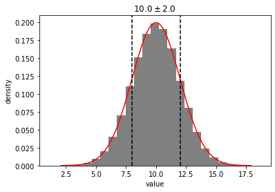
g = distl.gaussian(10, 2)
out = g.plot(show=True)
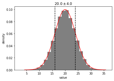
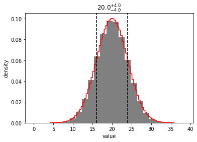
multiplying a Gaussian distribution by a float or integer treats that float or integer as a Delta distribution. In this case, it is able to return another Gaussian distribution. When unable to return a supported distribution type, a Composite distribution will be returned instead.
print(2*g)
<distl.gaussian loc=20.0 scale=4.0>
print(g*2)
<distl.gaussian loc=20.0 scale=4.0>
out = (g*2).plot(show=True)
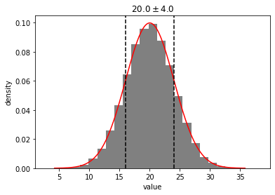
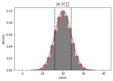
Note that this gives us the same resulting distribution as if we defined a Delta distribution manually and multiplied by that.
d = distl.delta(2)
print(g*d)
<distl.gaussian loc=20.0 scale=4.0>
out = (g*d).plot(show=True)
If we multiply in the other order, we'll get a Composite distribution, but see that it gives us the same resulting sample.
print(d*g)
<distl.delta loc=2.0> * <distl.gaussian loc=10.0 scale=2.0>
out = (d*g).plot(show=True)
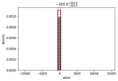
Note that since the floats/integers are treated as distributions, 2*g is not equivalent to g+g (note the change in the x-limit scale on the plot below compared to those above).
print(g+g)
<distl.gaussian loc=10.0 scale=2.0> + <distl.gaussian loc=10.0 scale=2.0>
out = (g+g).plot(show=True)
Supported Operators
- multiplication
- division
- addition
- subtraction
- np.sin, np.cos, np.tan
(for and/or logic, see these examples)
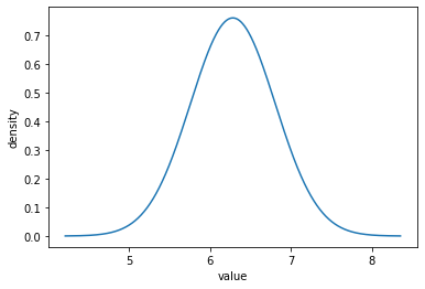
g = distl.gaussian(2*np.pi, np.pi/6)
print(np.sin(g))
sin(<distl.gaussian loc=6.283185307179586 scale=0.5235987755982988>)
out = g.plot_pdf(show=True)
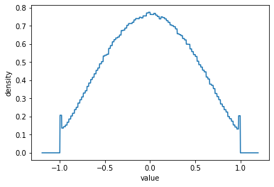
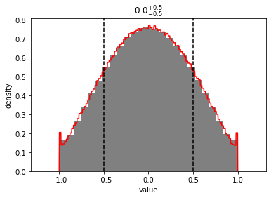
out = np.sin(g).plot_pdf(show=True)
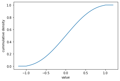
out = np.sin(g).plot_cdf(show=True)
out = np.sin(g).plot(show=True)
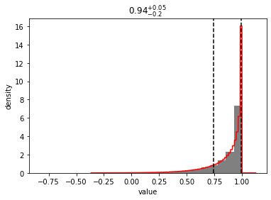
out = np.cos(g).plot(show=True)
out = np.tan(g).plot(show=True)