import distl
import numpy as np

Multivariate Gaussian

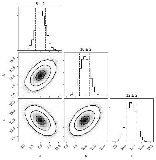
First we'll create a multivariate gaussian distribution by providing the means and covariances of three parameters.

mvg = distl.mvgaussian([5,10, 12], 
                       np.array([[ 2,  1, -1], 
                                 [ 1,  2,  1], 
                                 [-1,  1,  2]]),
                       allow_singular=True,
                       labels=['a', 'b', 'c'])

mvg.sample()

array([ 7.99080238, 11.46448835, 10.47368597])

mvg.sample(size=5)

array([[ 4.52006299, 10.4107841 , 12.89072111],
       [ 4.6485998 ,  9.62679128, 11.97819148],
       [ 3.36823516,  9.32211349, 12.95387833],
       [ 6.51815561, 12.77600097, 13.25784536],
       [ 2.61171535,  6.80428169, 11.19256635]])

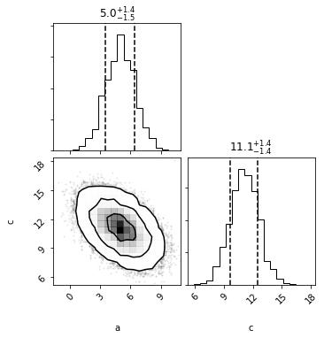
and plotting will now show a corner plot (if corner is installed)

fig = mvg.plot(show=True)

png

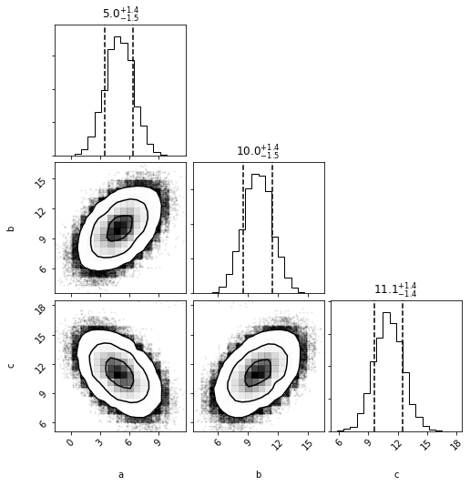
Multivariate Histogram

we can now convert this multivariate gaussian distribution into a multivariate histogram distribution (alternatively we could create a histogram directly from a set of samples or chains via mvhistogram_from_data.

mvh = mvg.to_mvhistogram(bins=15)

fig = mvh.plot(show=True, size=1e6)

png

np.asarray(mvh.density.shape)

array([15, 15, 15])

Now if we access the means and covariances, we'll see that they are slightly different due to the binning.

mvh.calculate_means()

array([ 4.98034068,  9.97330153, 11.06628499])

mvh.calculate_covariances()

array([[ 2.14195908,  0.99110644, -1.00913987],
       [ 0.99110644,  2.12047209,  0.99845476],
       [-1.00913987,  0.99845476,  2.14286097]])

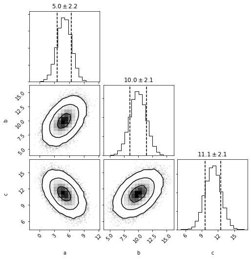
If we convert back to a multivariate gaussian, these are the means and covariances that will be adopted (technically not exactly as they'll be recomputed from another sampling of the underlying distribution).

mvhg = mvh.to_mvgaussian()

fig = mvhg.plot(show=True)

png

mvhg.mean

array([ 4.96639469,  9.9626855 , 11.05921629])

mvhg.cov

array([[ 2.15170257,  0.99878184, -1.01242674],
       [ 0.99878184,  2.12055321,  0.9920415 ],
       [-1.01242674,  0.9920415 ,  2.14125743]])

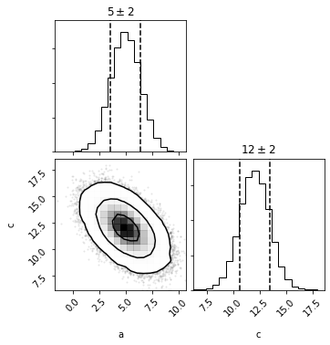
Take Dimensions

mvg_ac = mvg.take_dimensions(['a', 'c'])

mvg_ac.sample()

array([ 6.01363707, 13.52263276])

out = mvg_ac.plot(show=True)

png

out = mvh.take_dimensions(['a', 'c']).plot(show=True)

png

Passing a single dimension to take_dimension

If you pass a single-dimension to take_dimension, then the univariate version of the same type is returned instead. See the "Converting to Univariate" section below for examples directly calling to_univariate.

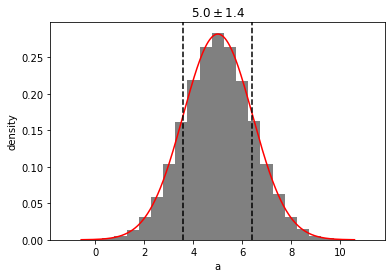
out = mvg.take_dimensions(['a']).plot(show=True)

png

Slicing

Slicing allows taking a single dimension while retaining all underlying covariances such that the resulting distribution can undergo math operations, and/or logic, and included in distribution collections. For more details, see the slice examples.

mvg_a = mvg.slice('a')

mvg_a.sample()

6.160840301541623

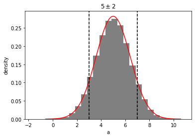
out = mvg_a.plot(show=True)

png

mvg_a.multivariate

<distl.mvgaussian mean=[5, 10, 12] cov=[[ 2  1 -1]
 [ 1  2  1]
 [-1  1  2]] allow_singular=True labels=['a', 'b', 'c']>

Converting to Univariate

There are methods to convert directly to the univariate distribution of the same type as the univariate:

When acting on a Multivariate, the requested dimension must be passed.

mvg.to_univariate(dimension='a')

<distl.gaussian loc=5.0 scale=1.4142135623730951 label=a>

Whereas a MultivariateSlice converts using the sliced dimension

mvg_a.to_univariate()

<distl.gaussian loc=5.0 scale=1.4142135623730951 label=a>